In the Connection tab you can configure the sensors associated with a module.

Use the button![]() to add sensors manually and the button
to add sensors manually and the button![]() to remove sensors. You can also use the search function
to remove sensors. You can also use the search function![]() to list all available sensors in the network. Sensors that were found but are not
required for the configuration can be removed from the table. For sensors in a buddy
mode group, the master of the group is displayed.
to list all available sensors in the network. Sensors that were found but are not
required for the configuration can be removed from the table. For sensors in a buddy
mode group, the master of the group is displayed.
The following settings can be configured for each sensor:
Name
This name is used internally by ibaPDA for identification and is not related to the sensor settings. When a new sensor is detected, the respective serial number is used as the default setting.
IP Address
The IP address at which a sensor can be reached for communication. By using the ![]() button, the web interface of the sensor can be opened (standard web browser).
button, the web interface of the sensor can be opened (standard web browser).
X offset
The offset of a sensor in mm along the axis of the sensor’s laser line. The X offset value is retrieved from the sensor and saved in the sensor if the read-only module setting is disabled. This parameter is required when constructing a profile based on the data of multiple sensors. It can be measured manually or using ibaPDA when acquiring a test profile of all sensors (see below).
Note |
|
|---|---|
|
The X offset value must be a multiple of the resolution of the Gocator module. For example, if the resolution is set to 500 µm, the value 10.486 mm is automatically set to 10.500 mm. |
|
Z offset
The offset of a sensor in height direction. The value is retrieved from and stored in the sensor if the read-only module setting is disabled. Typically, this value is obtained by using the sensor's alignment function (see below).
Angle
The angle between the object to be measured and the sensor plane. The value is retrieved from and stored in the sensor if the read-only module setting is disabled. Typically, this value is obtained by using the sensor's alignment function (see below).
Bank
The number of the bank to which the sensor is assigned. A bench is a subgroup of sensors that can generate a laser line and measure the profiles simultaneously without interfering with each other. The following illustration shows an arrangement of 6 sensors measuring a slab:
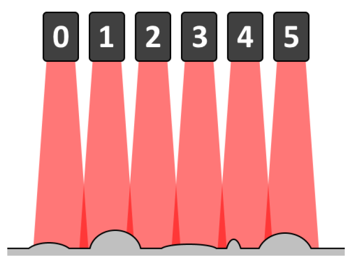
In the ideal case, if the sensors can be positioned exactly next to each other, there is no overlap of the laser lines. However, if the measured object has high contours, the covered width of the laser line is smaller than with low contours. If the entire slab with its high and low contours is to be covered, the sensors must be positioned with a certain overlap of their laser lines.
If all sensors were to generate a laser line and measure a profile at the same time, the laser line from sensor 1, for example, would interfere with the laser line from sensor 0 and thus also influence the measurement data. Sensor 1 would also interfere with sensor 2 at the same time. To prevent this, the exposure can be staggered over time in groups, the so-called banks.
Example:
Assuming, you want to obtain a full profile every millisecond (i. e. continuous measurements can be divided into time windows of 1 ms), whereby the exposure time (i. e. the time required to perform a valid profile measurement) of a laser is 400 µs. For this purpose, in each time window, sensor 0 can generate the laser line and measure the profile from 0 µs to 400 µs, while sensor 1 does this for the range from 400 µs to 800 µs. This leaves a span of 200 µs and there is no longer any mutual interference, as the sensors, which would normally overlap, generate their laser lines at different times. Since sensor 1 and sensor 2 also overlap, the time-division multiplexing method should also be used for the exposure time. Sensor 0 and sensor 2, on the other hand, can generate the laser line at the same time as they do not overlap.
In the figure above, this implies that sensors 0, 2 and 4 can generate the laser line at the same time (e.g. in the subslot from 0 µs to 400 µs) and sensors 1, 3 and 5 can generate the laser line at a different time (e.g. in the subslot from 400 µs to 800 µs). Sensors 0, 2 and 4 form the first bank, while sensors 1, 3 and 5 form the second bank.
Since the Gocator sensors work independently of each other and do not know each other, this setting is not saved in the sensor.
Exposure time
The time required to perform a valid profile measurement for this sensor. This value is retrieved from and stored in the sensor. This value is normally obtained by configuring the sensor via its web interface (by checking the live image).
Aligned
A read-only field that indicates whether the sensor has been successfully aligned. This field is updated when a sensor is automatically added via the discovery function or a connection test is performed.
Checking a sensor’s status and connection
To check whether a connection to a sensor can be established or to obtain basic diagnostic
information, select the respective sensor and click on the button . To check the connection to all listed sensors, click on the button
 .
.
Select the Status tab below the list. When the connection is checked, the current status, the model, the firmware version, the serial number of the sensor and, if applicable, the status information of its buddy sensors are displayed.
Aligning a sensor (not available in read-only mode)
Before the sensors can be used for a measurement, the Z offset and Angle values must be configured correctly. To do this, place a flat surface underneath
the sensor (i.e. the position on which the measurement object will later be placed)
and click the  button to align the selected sensor or the
  button to align all sensors. The Z offset and Angle values are updated automatically.
Acquiring a single profile
Although the X offset parameter is also set when the sensors are aligned, this will not initially be the
correct value: "X-Offset" refers to the distance from a sensor to a reference sensor.
However, as the sensors do not know each other, it is not possible to determine this
value automatically. However, the following method makes it possible to determine
a relatively accurate value for "X-Offset": by clicking the  button (for a single sensor or sensors in buddy mode) or the
  button (for all sensors), the current profile is retrieved and displayed in the Alignment tab.

The graphic above shows 2 aligned sensors; however, the "X-Offset" value is not yet set correctly. As the sensors overlap, their profiles should partially match. In this example, the area circled in red and the area circled in blue should overlap. Markers can be used to measure the distance between the two areas in the graphic; this value can then be used as the "X offset" for one of the sensors. If this value is entered in the sensor table and then the profiles are queried again, the following result is obtained:

The profiles now overlap correctly and the correct value for X-Offset has been found.
Note |
|
|---|---|
|
Markers can only be made visible after exiting live mode. You have the following options for exiting live mode: 1. Right-click in the graph (context menu) - select Live mode or 2. Zoom into the graph or 3. Press <F6>. To return to live mode, press <F6> again or use the context menu. |
|
As soon as the X offset parameter has been adjusted, the number of signals must be updated. To perform the
update, click on the button . Based on the resolution of the module and the X offset parameters of all sensors, ibaPDA generates the required number of signals. Each signal corresponds to a single data
point of the entire profile.
. Based on the resolution of the module and the X offset parameters of all sensors, ibaPDA generates the required number of signals. Each signal corresponds to a single data
point of the entire profile.