Some bandpass-filtered characteristics require parameters to enable the trend to be calculated by the CMU. These parameters can be defined on the CMU calculations tab.
Calculation example for a filtered RMS value
For an RMS 10-2000 the “Lower frequency limit” is set to 10 Hz and the “Upper frequency limit” to 2000 Hz under Parameters. This gives a characteristic value for activity in this frequency range for monitoring.
Enable
Switch to enable (green) or disable (gray) the calculation.
Calculation
If you have used a particular trend from the library, this field is pre-selected. This setting can not then be changed.
Predefined calculation methods for selection include:
-
Average [Avg]
-
Crest factor [CF]
-
ISO [ISO]
-
K(t)
-
Maximum [Max]
-
Median [Med]
-
Minimum [Min]
-
Peak to peak [PP]
-
Effective value [RMS]
Multiplier
An optional additional factor can be specified here, by which the trend value is multiplied after the actual calculation.
Parameters
Note:
Fixed parameters are assigned for the trend and can be changed if required. When changing existing trends, the trend history with the previous settings will remain unchanged and not recalculated. The trend name is not adjusted in case of changing parameters. It should be adjusted manually to match the settings again.
Overview of calculation parameters:
-
Lower frequency limit
-
Order analysis
-
Order harmonics
-
Upper Frequency limit
Note |
|
|---|---|
|
For the RMS trends you can enter 0 Hz as Upper frequency limit. In case of an ibaCMU-S half the sampling rate will be exported for Upper frequency limit which corresponds to the maximum frequency (fmax) in the spectrum. In case of an ibaDAQ 0 Hz will be exported. ibaPDA then generates a high-pass-filter with Lower frequency limit. |
|
Damage pattern calculation for components
Multiple virtual trends are calculated for each component. A predefined damage pattern is used as the basis for calculation of these trends, e. g. FFT inner race, ENV outer race etc. Calculation and configuration of the damage pattern is described here using the example of “Envelope curve inner race” (ENV inner race).
The relevant damage pattern calculation and also the calculation type (average, min, max, etc.) are displayed in the CMU calculation section on the ENV inner race harmonics and ENV inner race sidebands tabs. For example, this means that the average for all harmonics is calculated and used to plot the trend. The multiplier enables the harmonics, for example, to be given greater weighting than the sidebands.
The Damage patterns <Edit> button opens a listing of the harmonics of the component's defect frequency or the sidebands of these harmonics.
On the ENV inner race harmonics tab you can use this dialog to set up tolerances for the 1st to 8th harmonics in order to define a band width to be searched for the calculated value, e. g. the maximum.
On the ENV inner race sidebands tab you can use this dialog to enable or disable up to 8 sidebands for each of the 1st to 8th harmonics. Furthermore, you can set the band width to be searched for the maximum by specifying the tolerance.
The Tolerance entry applies as a symmetrical value given in percent to the left and to the right of the damage frequency (bandwidth = 2 * tolerance).
Example:
If the defect frequency is 50 Hz and the band width is set to 0.1 (10 % of the defect frequency), you should enter 5 % for tolerance. The frequency range from 47.5 Hz to 52.5 Hz will be considered (band width = 5 Hz).
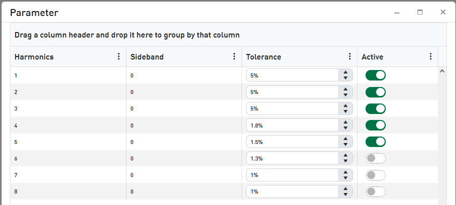
In this example the tolerance is 5 % for the fundamental and the next two harmonics. Consequently, the band width in Hz increases by rising frequencies.
If you want to get a comparable precision, i. e. a similar band width like for the fundamental even for the higher harmonics, then you have to decrease the tolerances for higher frequencies.

CMU correlation
Correlation is usually calculated using the correlation app. The values calculated there are also displayed here.
For more information about the correlation settings, see Correlation settings