The correlation module provides valuable support in highlighting correlations between vibration values and process parameters in virtual trends. This is especially useful where the vibration characteristic values for the plant depend on a process parameter but there is no link to damage. As soon as a component is dragged to the relevant workspace in the correlation window, all trends available under this component are loaded.
Note:
If a component from a high level, e.g. a plant or an aggregate group, is selected, the number of associated trends can be very high, which significantly increases the loading time. If the predefined number of trends is exceeded, loading is aborted. In this case, you can either increase the value or choose a component from a lower level, e.g. a component group.
Filter parameters
The entries are displayed, based on the filter parameters. The parameters are listed below.
|
From |
The start date for the time range to be used for calculation of the new correlation settings. The default value is one month in the past. |
|
To |
The end date for the time range to be used for calculation of the new correlation settings. The default value is the current date. |
|
Regression |
This refers to the regression method. In the current version, only “Linear regression” can be selected. |
|
Correlation signal |
A sensor can be dragged to this field from the plant. The trends that can be correlated are then listed below it. Selectable correlation signals:
|
|
Max. number of trends |
The maximum number of virtual trends that are simultaneously loaded. It may be necessary to increase this value if you have selected a larger plant unit, e.g. an aggregate. |
|
Total number |
Shows the number of virtual trends found for the selected plant component. Note: If a filter is set in one of the columns in the list, the number of rows displayed may be lower than the total number. |
|
Force overwrite |
Clicking on this button replaces the old values with the new ones. |
Meaning of regression parameters for linear regression
|
P1 |
Slope of the regression line determined |
|---|---|
|
P2 |
Maximum value of the correlation signal in the calculation period. The virtual trends are converted to this value. |
|
R^2 (R2) |
This parameter is referred to as the coefficient of determination and is between 0 and 1. Higher values indicate a higher linear relationship and show a higher “quality” of regression. 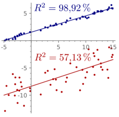 Source: https://commons.wikimedia.org/ At values above 0.5 the regression can bring an improvement in the trend values (especially for trends calculated from the envelope curve such as roller bearing trends), while at values below 0.5 the correlation should not be used. |
The pP1, pP2, and pR^2 columns show the correlation values from earlier calculations, if they have been performed. If the calculated parameters are unsatisfactory, they can be edited manually. To do this, select the checkbox in the Custom column. Clicking on the <Submit all> button permanently saves the new values. The <Remove all> button excludes these values from the correlation calculation. This operation does not delete the trends themselves.
No matter how many virtual trends are loaded in the background, the <Submit visible items> button only applies the values that are actually visible in the list. All other limits remain unchanged.
The Virtual trend type tab shows all trend types for which the correlation is possible. The trend types that are checked are recommended for the correlation.
Side note: How does correlation work?
Let us assume that the trend calculation for a vibration sensor (e.g. an RMS value) depends to a great extent on the motor speed. In this case, the RMS level increases with an increasing motor speed and, conversely, the RMS value falls as the motor speed reduces.
This situation means that a higher RMS level cannot automatically be attributed to a mechanical problem. To standardize the RMS value with the motor speed, we can use CMU correlation.
Linked to the above example, we can assume two signals:
-
The motor speed (also known as the independent variable in the static term or the X value)
-
The RMS value (also known as the dependent variable in the static term or the Y value)
Based on these two values, we can now calculate a line that best represents the data points.
This line is plotted in purple in the figure below. The calculation provides the parameter P1, which specifies the slope of the line, and the parameter P2, which corresponds to the highest measured motor speed in the data points, as well as the value R2, which indicates how well the line represents the data points.
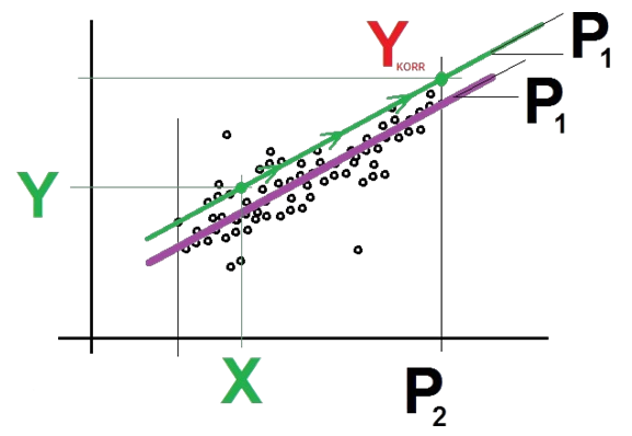
For the correlation process, the CMU starts with a new calculation of the vibration signal and the motor speed. These new values are X and Y. The CMU then makes the following calculation:
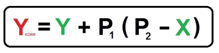
The calculation results in a shift in the originally calculated RMS value to a higher RMS value YCORR at a higher motor speed P2. In principle, this simulates measurement at a higher shaft speed.
The correlation principle means that the RMS trend is slightly smoother (less variance) as it no longer depends so much on the motor speed.