A value axis can contain several spectra. Using the legend, you can change the value axis used by a spectrum by changing the sequence of the signals. A value axis can be deleted via its context menu. This also deletes all spectra on this axis. You can also display the settings for the value axis via the context menu.

Settings for type, scaling and view correspond to the usual settings in ibaPDA and are self-explanatory.
Scaling
Linear, decibel or logarithmic can be set as scale type. This scale type is applied to the appearance of single spectrum, waterfall and contour.
Amplitude scaling
Depending on the requirements for the visualization, it may be useful to either emphasize or suppress the amplitudes for the display. The following methods are available:
-
-
Peak-to-peak Amplitude values are practically multiplied by a factor of two
-
RMS Amplitude values are practically divided by the root 2, thus moving closer to the RMS value.
-
Percentage of signal The scaling of the amplitude values is defined as a percentage of a signal. Select the signal in the Reference signal for percentage field.
-
Percentage of band peak The scaling of the amplitude values are based on the peak in a specific band. Enter the band number in the Band number for percentage field.
-
Scaling mode
-
Dynamic auto scale: if you enable this option, the scaling is always adjusted to the highest and lowest signal amplitudes in the graph (in both directions).
-
Dynamic auto scale (only for enlarging): When you enable this option, the scaling is continuously adjusted with the highest signal amplitudes. If the amplitudes go beyond the trend view again, the scaling still remains unchanged.
-
Manual scale: if this option is selected, the Min and Max scale values can be manually entered or selected from the field next to it. Beside a static value, you can also use any known measured or virtual analog signal configured in the I/O manager.
Note |
|
|---|---|
|
If Decibel is selected, the values of the manual scale nevertheless relate to the linear axis. The resulting decibel values are shown next to them.
|
|
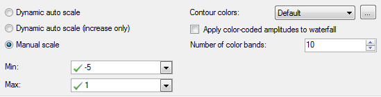
Color settings
You can choose one of the prepared color schemes for the contour colors (default, grey, jet-white, jet or heat). If you do not like any of the offered color schemes, you can design your own color schemes. To do this, click on the <...> button and the Manage perspectives dialog opens. Here you can define new color schemes or change existing ones.
In addition, the colors of the contour view can also be applied to the waterfall view. To do this, enable the Apply color-coded amplitudes to waterfall option. The number of color bands defines the color resolution. A maximum of 50 color bands is possible.

Note |
|
|---|---|
|
If Apply color-coded amplitudes to waterfall is enabled, custom value bands are displayed only in the spectrum graph. |
|
Spectrum x
By default, a Spectrum 1 tab is available. These settings are used to process a new signal that is dragged into the FFT view. You can drag multiple signals into an FFT view. If the signals share the same value axis, you will find a separate tab for each signal or spectrum. In the properties, the settings for each spectrum can be changed individually. If each signal or spectrum has its own value axis in the display, each spectrum in the tree structure on the left gets its own node for the value axis.
No calculation profile can be configured in the FFT view of ibaAnalyzer-InSpectra. A profile can only be configured for the data acquisition in ibaPDA without ibaInSpectra. This option is only used for the visualization. The results cannot be acquired. The FFT calculation profile, however, is compatible with InSpectra profiles.
Input
-
Select Data Source to specify the signal or InSpectra module to be displayed. If you have already dragged the signal into the display via drag & drop, the field is already filled in.
-
You only need to enter a Speed Source if you want to perform speed-dependent analyses or work with the order spectrum.
FFT calculation profile
The way in which ibaPDA calculates an FFT is defined in so-called profiles. A profile is a collection of various parameters that are relevant to an FFT.
Each spectrum can be calculated with a different profile. You can define as many profiles as you wish and save them in the system via the export function. You can also import saved profiles into a spectrum.
In the profiles, parameters are defined, including
-
Sensor data (important for vibration measurements)
-
Spectrum type (e.g. integrate, differentiate)
-
Speed data (important for order analysis)
-
Number of samples and lines, overlap
-
Basic calculation rules for the FFT (e.g. calculation mode, averaging, window type)
The button <Configure profile> opens the configuration dialog for profiles. The buttons <Export profile> and <Import profile> below can be used to export and import profiles.

The calculation parameters and their meaning are explained in the ibaInSpectra manual in chapter Setting calculation parameter.
The information next to the “Profile...” buttons describes the influence of the acquisition parameters:
-
Delta frequency: Shows the frequency steps between the results of the division of maximum frequency by bin count.
-
Max. update rate: Time required for update of the FFT view depending on bin count and overlap factor.
To avoid having to look at the properties to see the profile parameters, the display shows the Spectrum Parameter Table. This table is part of the FFT view and can be activated via the drop-down menu in the FFT view. The parameters from the calculation profile shown in the table can be defined in the Spectrum Parameter Table node in the FFT view properties. See chapter Spectrum parameter table
View
A spectrum can be visualized in four different ways:
-
Lines,
-
Bars,
-
Curve or
-
Dots
The inner area of a spectrum can be filled with a transparent or opaque color. The figure below shows the four types of spectra visualization, all filled transparently.
  |
  |
The option Improve isometric visibility is used to make spectra opaque. This makes some effects in the waterfall view more visible.