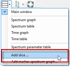
With a slice view, you can essentially represent the chronological sequence of an FFT for a selected marker position. The amplitude profile of a frequency therefore becomes clear, especially in conjunction with the isometric waterfall view. You add a slice view using the drop-down menu for the FFT display.

The slice view can operate in two modes:

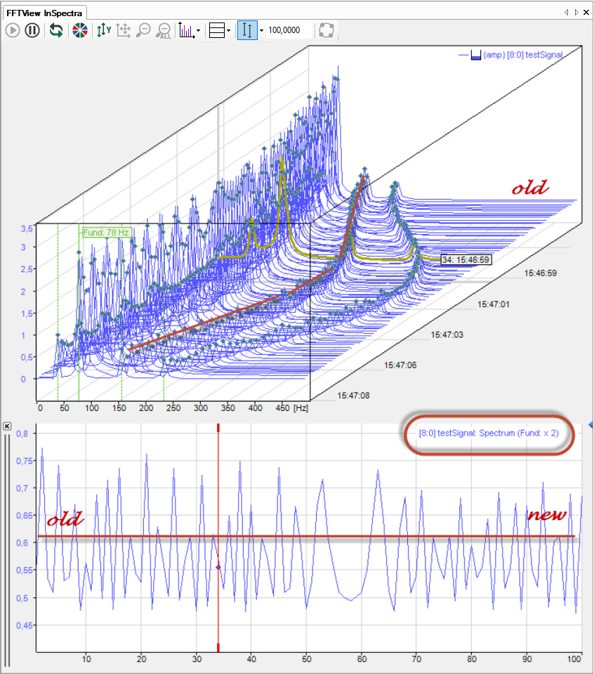
• In Spectrum Mode you can monitor a spectrum value that changes over time:

  • The temporal dimension corresponds to the number of planes in the waterfall view. The highest-numbered plane contains the most recent data (front plane). The scale of the X-axis shows the plane number.

  • The frequency dimension is specified by an interactive marker or a configured marker, which is connected to a signal, e.g., a speed signal.

• In Marker Mode you can monitor a frequency value that changes over time:

  • Here again, the temporal dimension corresponds to the number of planes.

  • Application example: Tracking a speed marker to show the speed history.

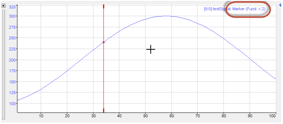
The mode of the slice view is also displayed in the signal legend.

You can add multiple slice views for different applications.

Once defined, the slice views are listed in the drop-down menu and can also be displayed, hidden and deleted there.

The slice view is specified by a marker. In the properties of the slice view, you can select any defined marker, including any available harmonic markers. You can also quickly switch between the different markers in the context menu on the slice view.

In addition, each slice view has its own interactive marker. You can link the interactive marker with the currently selected plane in the waterfall view with the “Link markers with waterfall” option. Note that the position of the interactive markers in the slice view always corresponds to one plane in the waterfall view.